flowchart LR
  A[Data Preparation] --> B[Data Summary]
  B --> C{Data Cleaning}
  C --> D[Market Overview Visualization 1: Trend of Average Unit Prices by Planning Region]
  C --> E[Market Overview Visualization 2: Popularity by Type of Sale]
Take-home Exercise 1:Singapore Private Residential Market

Task
In this Take Home Exercise, a few compelling and insightful data visualizations for the Singapore private residential market and its sub-markets for the first quarter of 2024 are created using Quarto.
Data Preparation
Data Source: private residential property transaction data from 1st January 2023 to 31st March 2024
Loaded necessary libraries and set the working directory to source transaction data. Aggregated CSV files, collating rows to form a complete dataset. Performed initial data summary, extracting transaction count, date range, unique property types, and regions. Cleaned data, replacing empty values with NAs and converting numeric fields for insightful analysis.
Code
pacman::p_load(ggplot2,lubridate,ggrepel, patchwork,
               ggthemes, hrbrthemes,
               tidyverse)

setwd("C:/kekekay/ISSS608-VAA/takehome/data")
full_data <-  list.files(
                    pattern = "*.csv",
                    full.names=T) %>%
                    lapply(read_csv) %>%
                    bind_rows()
Data Summary
Code
# data summary
total_transactions <- nrow(full_data)
date_range <- range(full_data$`Sale Date`, na.rm = TRUE)
property_types <- unique(full_data$`Property Type`)
total_property_types <- length(property_types)
region<- unique(full_data$`Planning Region`)
area<- unique(full_data$`Planning Area`)
Total Transactions:26806
Date Range is from 01 Apr 2023 to 31 Oct 2023
Total Unique Property Types: 6
List of Property Types: Condominium, Executive Condominium, Terrace House, Semi-Detached House, Apartment, Detached House

Planning Region: Central Region, East Region, North Region, North East Region, West Region
Planning Area: Bukit Merah, Bedok, Yishun, Sengkang, Hougang, Bukit Timah, Marine Parade, Clementi, Woodlands, Serangoon, Tanglin, Tampines, Kallang, Rochor, Novena, Punggol, Sembawang, Downtown Core, Bishan, Jurong West, Pasir Ris, Queenstown, Bukit Panjang, Bukit Batok, Museum, Newton, Southern Islands, Toa Payoh, Choa Chu Kang, Geylang, River Valley, Orchard, Singapore River, Outram, Tengah, Ang Mo Kio, Jurong East, Mandai, Sungei Kadut, Changi, Paya Lebar
Data Cleaning
Code
cleaned_data <- full_data %>%
  mutate(across(c(`Nett Price($)`, `Area (SQM)`, `Unit Price ($ PSM)`), ~replace(., . == "" | . == "-", NA))) %>%
  mutate(
    `Transacted Price ($)` = as.numeric(gsub(",", "", `Transacted Price ($)`)),
    `Area (SQFT)` = as.numeric(`Area (SQFT)`),
    `Unit Price ($ PSF)` = as.numeric(gsub(",", "", `Unit Price ($ PSF)`)),
    `Sale Date` = dmy(`Sale Date`),
    `Area (SQM)` = as.numeric(`Area (SQM)`),
    `Unit Price ($ PSM)` = as.numeric(gsub(",", "", `Unit Price ($ PSM)`)),
    `Nett Price($)` = ifelse(is.na(`Nett Price($)`),
                             `Area (SQM)` * `Unit Price ($ PSM)`,
                             as.numeric(gsub(",", "", `Nett Price($)`)))
  )
Code Explanation
Use of
across: Theacross()function is applied to check and replace empty or placeholder values across specified columns. It replaces any empty strings or ‘-’ withNA.Cleaning and Converting Data: After the placeholders are handled, the script then cleans up currency and area fields, removing commas and converting them to numeric where necessary.
Conditional Calculation for
Nett Price($): After ensuring all data types are correct and placeholders are handled, it calculatesNett Price($)where needed.
Market Overview Visualization 1: Trend of Average Unit Prices by Planning Region
Code
p1 <- cleaned_data %>%
  filter(`Planning Region` == "Central Region") %>%
  group_by(Month = floor_date(`Sale Date`, "month"), `Type of Sale`, `Property Type`) %>%
  summarize(Average_Price = mean(`Unit Price ($ PSM)`, na.rm = TRUE), .groups = 'drop') %>%
  ggplot(aes(x = Month, y = Average_Price, color = `Type of Sale`)) +
  geom_line() +
  scale_x_date(date_breaks = "3 month", date_labels = "%b %Y") +
  labs(
    title = "Central Region: Trend of Average Unit Prices Over Time",
    x = "Month",
    y = "Average Unit Price ($ PSM)"
  ) +
  facet_wrap(~ `Property Type`, scales = "free_y", strip.position = "bottom") +
  theme(
    plot.title = element_text(size = rel(1.5)),
    legend.position = "top",
    legend.text = element_text(size = rel(0.8)),
    panel.grid.major = element_line(color = "grey80"),
    panel.grid.minor = element_blank(),
    plot.margin = margin(10, 10, 10, 10),
    strip.text = element_text(size = rel(0.8)),  # adjust strip text size
    axis.text.x = element_text(size = rel(0.8), angle = 45, hjust = 1, vjust = 1),  # adjust x-axis text size
    axis.ticks.length = unit(-3, "pt"),  #aAdjust tick length
    panel.spacing = unit(1, "lines")  # adjust spacing between facets
  )

p1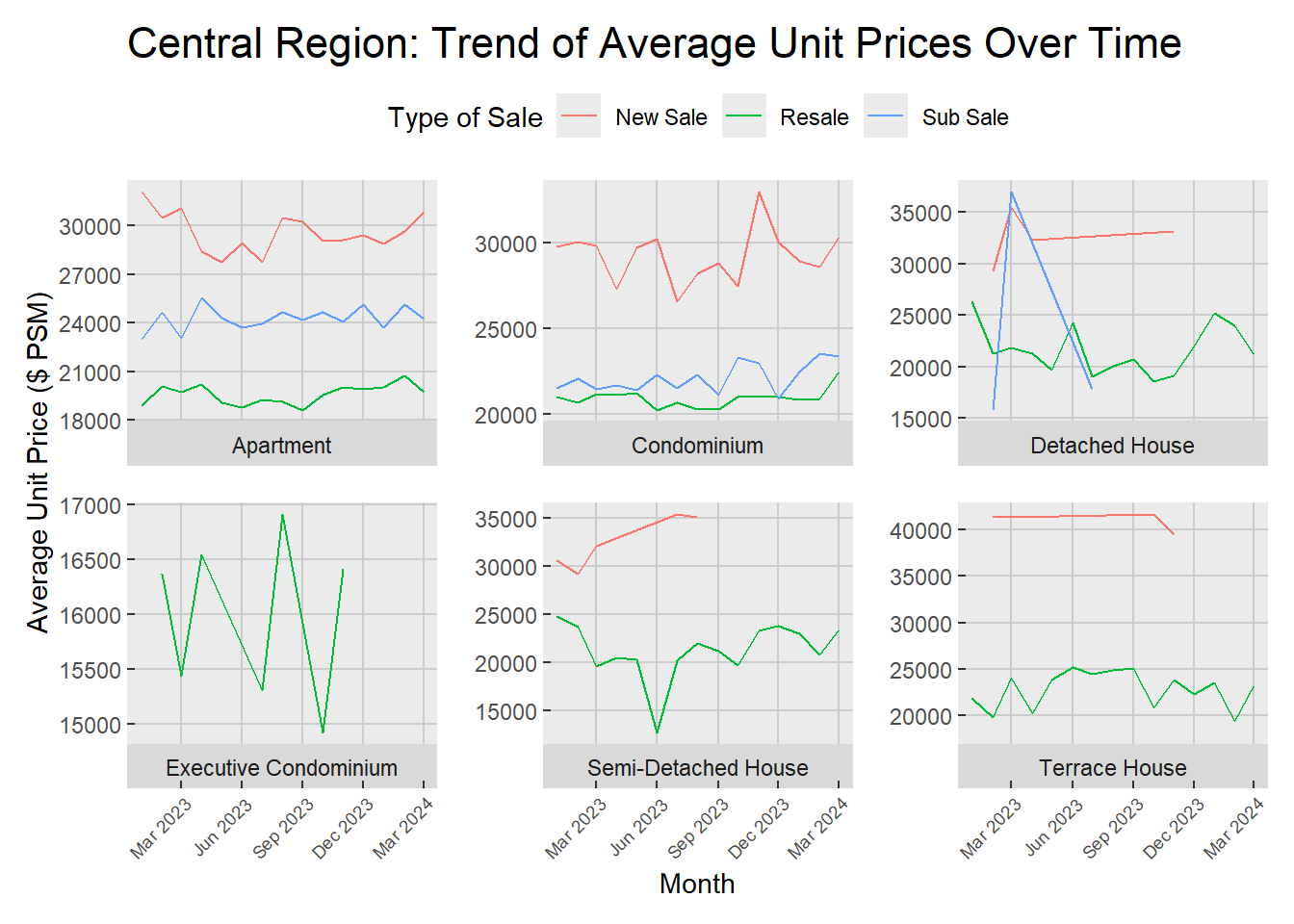
In the Central Region, Q1 2024 presents a stable pricing pattern for apartments, condominiums, and terrace houses, mirroring trends from the previous year. Conversely, detached houses experienced a significant rise in prices, followed by a pronounced dip, particularly within the sub-sale segment, which has now narrowed down to only resale transactions. It shows there was flutuation under Executive condominiums from March to December 2023, culminating in a complete absence of new sales in the subsequent quarter. Meanwhile, semi-detached houses witnessed a singular decline in June 2023, after which prices entered a gradual and steady climb, indicating a stabilizing market as progress through 2024.
Code
p2 <- cleaned_data %>%
  filter(`Planning Region` == "East Region") %>%
  group_by(Month = floor_date(`Sale Date`, "month"), `Type of Sale`, `Property Type`) %>%
  summarize(Average_Price = mean(`Unit Price ($ PSM)`, na.rm = TRUE), .groups = 'drop') %>%
  ggplot(aes(x = Month, y = Average_Price, color = `Type of Sale`)) +
  geom_line() +
  scale_x_date(date_breaks = "3 month", date_labels = "%b %Y") +
  labs(
    title = "East Region:Trend of Average Unit Prices Over Time",
    x = "Month",
    y = "Average Unit Price ($ PSM)"
  ) +
  facet_wrap(~ `Property Type`, scales = "free_y", strip.position = "bottom") +
  theme(
    plot.title = element_text(size = rel(1.5)),
    legend.position = "top",
    legend.text = element_text(size = rel(0.8)),
    panel.grid.major = element_line(color = "grey80"),
    panel.grid.minor = element_blank(),
    plot.margin = margin(10, 10, 10, 10),
    strip.text = element_text(size = rel(0.8)),
    axis.text.x = element_text(size = rel(0.8), angle = 45, hjust = 1, vjust = 1),
    axis.ticks.length = unit(-3, "pt"),
    panel.spacing = unit(1, "lines")
  )

p2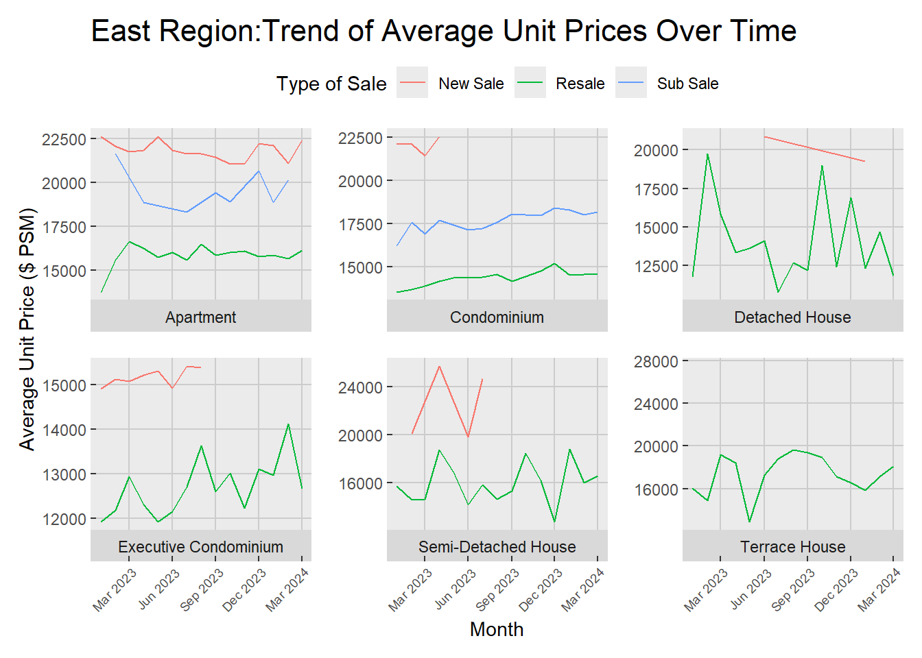
In East Region, Apartments, condominiums and terrace houses have shown relative price stability, with condominiums displaying a slight uprend. Detached houses have seen erratic price movements with a sharp rise followed by a decline in sub-sale prices. Executive condominiums display notable price swings throughout the year, overall, it still demonstrates an upward price trend. In contrast, semi-detached houses show a significant dip year-end but recover to a gentle upward trend.
Code
p3 <- cleaned_data %>%
  filter(`Planning Region` == "North East Region") %>%
  group_by(Month = floor_date(`Sale Date`, "month"), `Type of Sale`, `Property Type`) %>%
  summarize(Average_Price = mean(`Unit Price ($ PSM)`, na.rm = TRUE), .groups = 'drop') %>%
  ggplot(aes(x = Month, y = Average_Price, color = `Type of Sale`)) +
  geom_line() +
  scale_x_date(date_breaks = "3 month", date_labels = "%b %Y") +
  labs(
    title = "North East Region: Trend of Average Unit Prices",
    x = "Month",
    y = "Average Unit Price ($ PSM)"
  ) +
  facet_wrap(~ `Property Type`, scales = "free_y", strip.position = "bottom") +
  theme(
    plot.title = element_text(size = rel(1.5)),
    legend.position = "top",
    legend.text = element_text(size = rel(0.8)),
    panel.grid.major = element_line(color = "grey80"),
    panel.grid.minor = element_blank(),
    plot.margin = margin(10, 10, 10, 10),
    strip.text = element_text(size = rel(0.8)),
    axis.text.x = element_text(size = rel(0.8), angle = 45, hjust = 1, vjust = 1),
    axis.ticks.length = unit(-3, "pt"),
    panel.spacing = unit(1, "lines")
  )

p3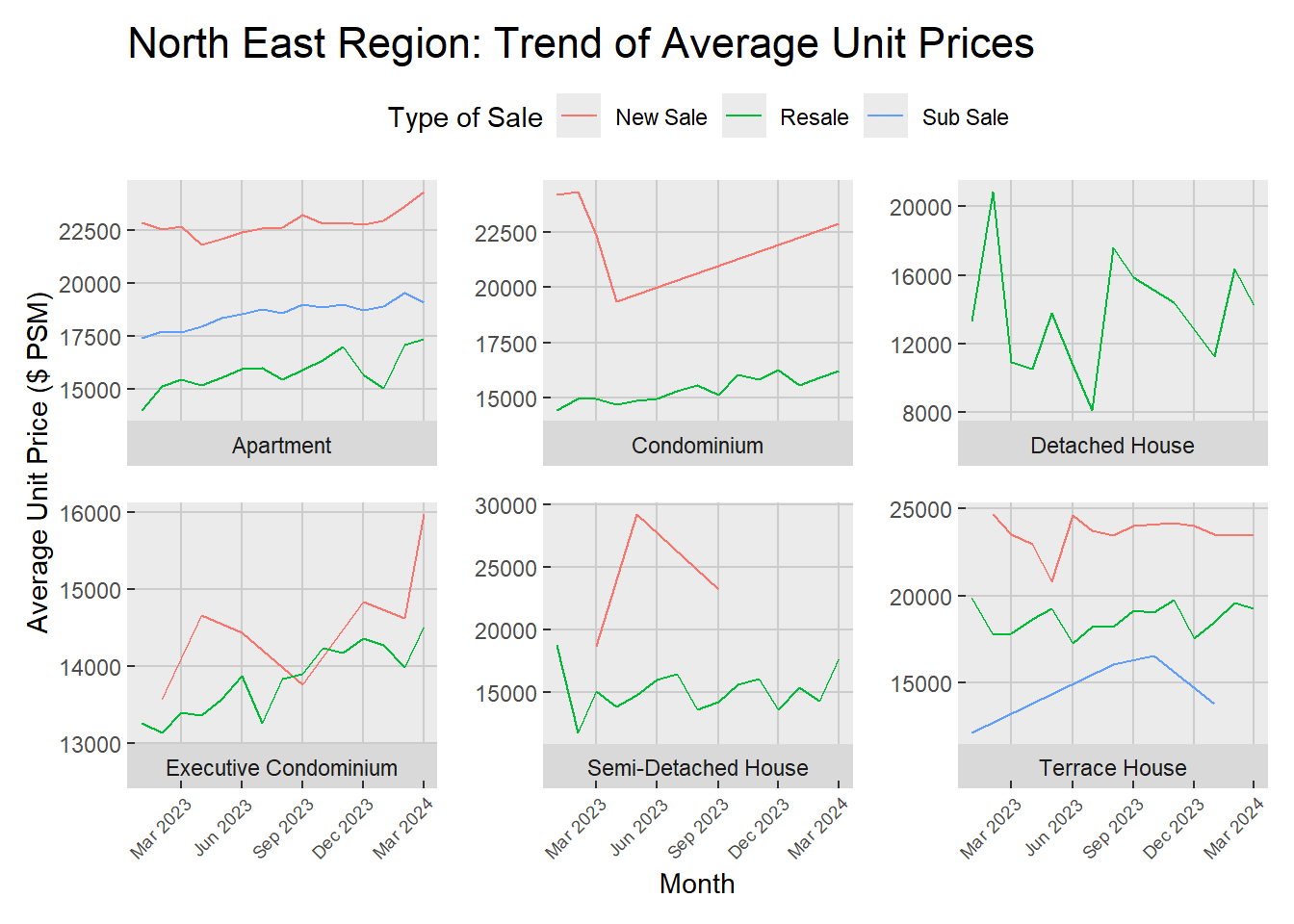
In the North East region, the fluctuation in the prices of detached houses is quite pronounced. Additionally, there’s a notable upward trend in the prices of executive condominiums, especially within the new sales category.
Code
p4 <- cleaned_data %>%
  filter(`Planning Region` == "North Region") %>%
  group_by(Month = floor_date(`Sale Date`, "month"), `Type of Sale`, `Property Type`) %>%
  summarize(Average_Price = mean(`Unit Price ($ PSM)`, na.rm = TRUE), .groups = 'drop') %>%
  ggplot(aes(x = Month, y = Average_Price, color = `Type of Sale`)) +
  geom_line() +
  scale_x_date(date_breaks = "3 month", date_labels = "%b %Y") +
  labs(
    title = "North Region:Trend of Average Unit Prices Over Time",
    x = "Month",
    y = "Average Unit Price ($ PSM)"
  ) +
  facet_wrap(~ `Property Type`, scales = "free_y", strip.position = "bottom") +
  theme(
    plot.title = element_text(size = rel(1.5)),
    legend.position = "top",
    legend.text = element_text(size = rel(0.8)),
    panel.grid.major = element_line(color = "grey80"),
    panel.grid.minor = element_blank(),
    plot.margin = margin(10, 10, 10, 10),
    strip.text = element_text(size = rel(0.8)),
    axis.text.x = element_text(size = rel(0.8), angle = 45, hjust = 1, vjust = 1),
    axis.ticks.length = unit(-3, "pt"),
    panel.spacing = unit(1, "lines")
  )

p4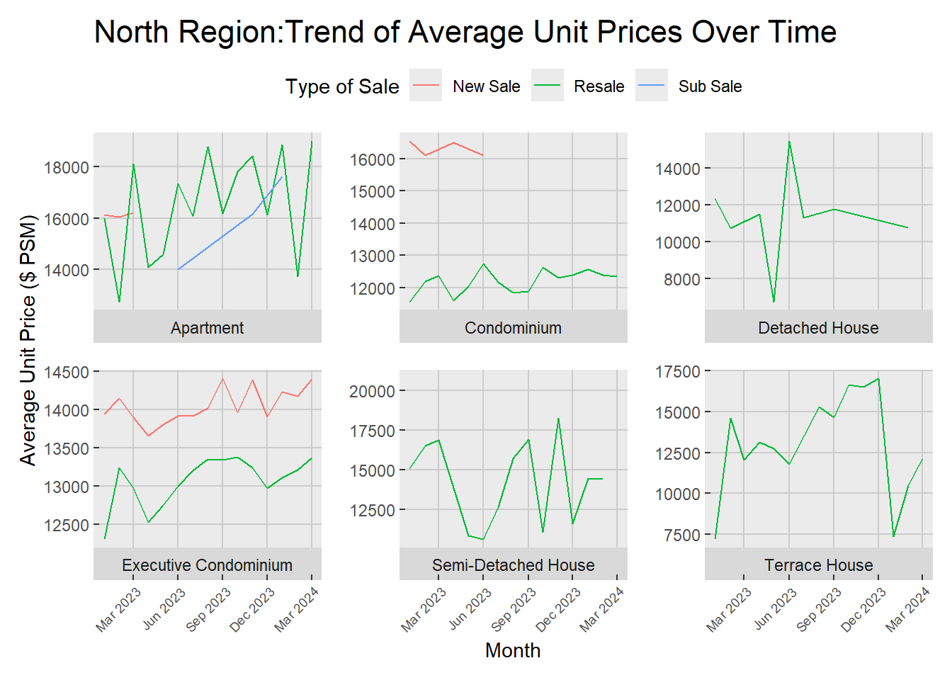
In the North Region, apart from condominiums, other property types display considerable instability. However, as of March 2024, apartments, executive condominiums, and terrace houses continue to exhibit an increasing price trend.
Code
p5 <- cleaned_data %>%
  filter(`Planning Region` == "West Region") %>%
  group_by(Month = floor_date(`Sale Date`, "month"), `Type of Sale`, `Property Type`) %>%
  summarize(Average_Price = mean(`Unit Price ($ PSM)`, na.rm = TRUE), .groups = 'drop') %>%
  ggplot(aes(x = Month, y = Average_Price, color = `Type of Sale`)) +
  geom_line() +
  scale_x_date(date_breaks = "3 month", date_labels = "%b %Y") +
  labs(
    title = "West Region:Trend of Average Unit Prices Over Time",
    x = "Month",
    y = "Average Unit Price ($ PSM)"
  ) +
  facet_wrap(~ `Property Type`, scales = "free_y", strip.position = "bottom") +
  theme(
    plot.title = element_text(size = rel(1.5)),
    legend.position = "top",
    legend.text = element_text(size = rel(0.8)),
    panel.grid.major = element_line(color = "grey80"),
    panel.grid.minor = element_blank(),
    plot.margin = margin(10, 10, 10, 10),
    strip.text = element_text(size = rel(0.8)),
    axis.text.x = element_text(size = rel(0.8), angle = 45, hjust = 1, vjust = 1),
    axis.ticks.length = unit(-3, "pt"),
    panel.spacing = unit(1, "lines")
  )

p5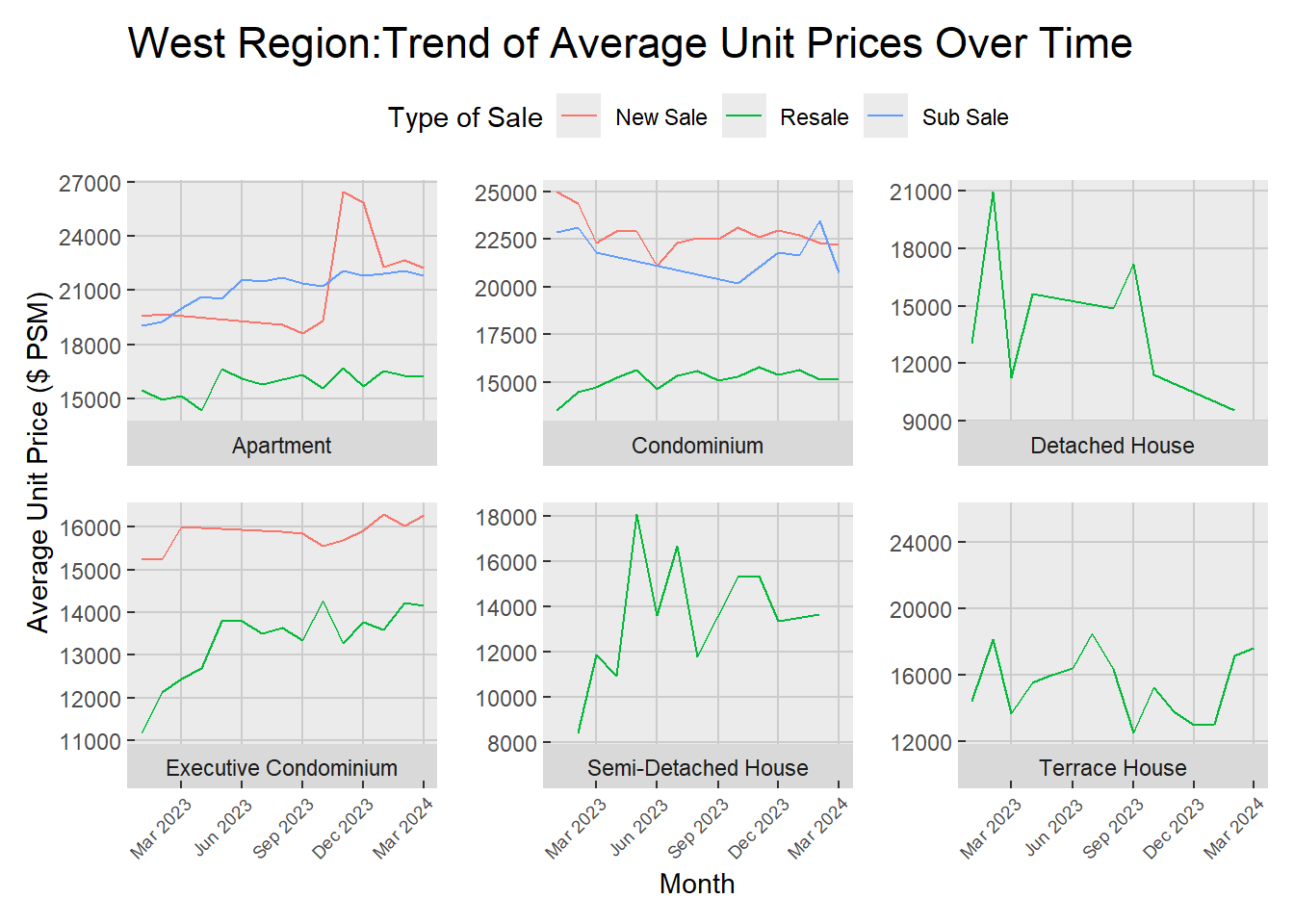
In the West Region, December 2023 marked a notable uptick in the prices of new sale apartments, surging from approximately $19,000 PSM to $26,000 PSM, before settling back at $22,000 PSM. Conversely, detached and semi-detached houses demonstrated a downward pricing trend.
In summary, the Central Region commands the highest unit prices across the board, while the North Region is distinguished by the lowest. Typically, new sales achieve higher prices than sub-sales and resales. However, an exception is noted in the North East Region, where terrace houses experience the lowest prices in sub-sales. Furthermore, the North East and North Regions are both exhibiting an upward price trend as we progress through Q1 of 2024.
Market Overview Visualization 2: Popularity by Type of Sale
Code
# number of transactions by type of sale
transactions_by_sale_type <- cleaned_data %>%
  count(`Type of Sale`) %>%
  mutate(Percentage = n / sum(n) * 100,
         Label = paste(`Type of Sale`, round(Percentage, 1), "%"))  # set label for each slice

# Custom colors for the pie slices
slice_colors <- c("New Sale" = "darkseagreen", "Resale" = "lavender", "Sub Sale" = "pink")

# Create the pie chart
pie_chart <- ggplot(transactions_by_sale_type, aes(x = "", y = Percentage, fill = `Type of Sale`)) +
  geom_col(width = 1) +  # this is to create a bar for each slice with a width that ensures no gaps
  coord_polar(theta = "y") +
  scale_fill_manual(values = slice_colors) +
  geom_text(aes(label = Label), position = position_stack(vjust = 0.5)) +  # add labels of each slice
  labs(
    title = "Popularity Overview by Type of Sale",
    x = NULL,
    y = NULL,
    fill = "Type of Sale"
  ) +
  theme_void() +
  theme(
    legend.position = "bottom",  # legend postion
    plot.title = element_text(hjust = 0.5)  # plot title position
  )

pie_chart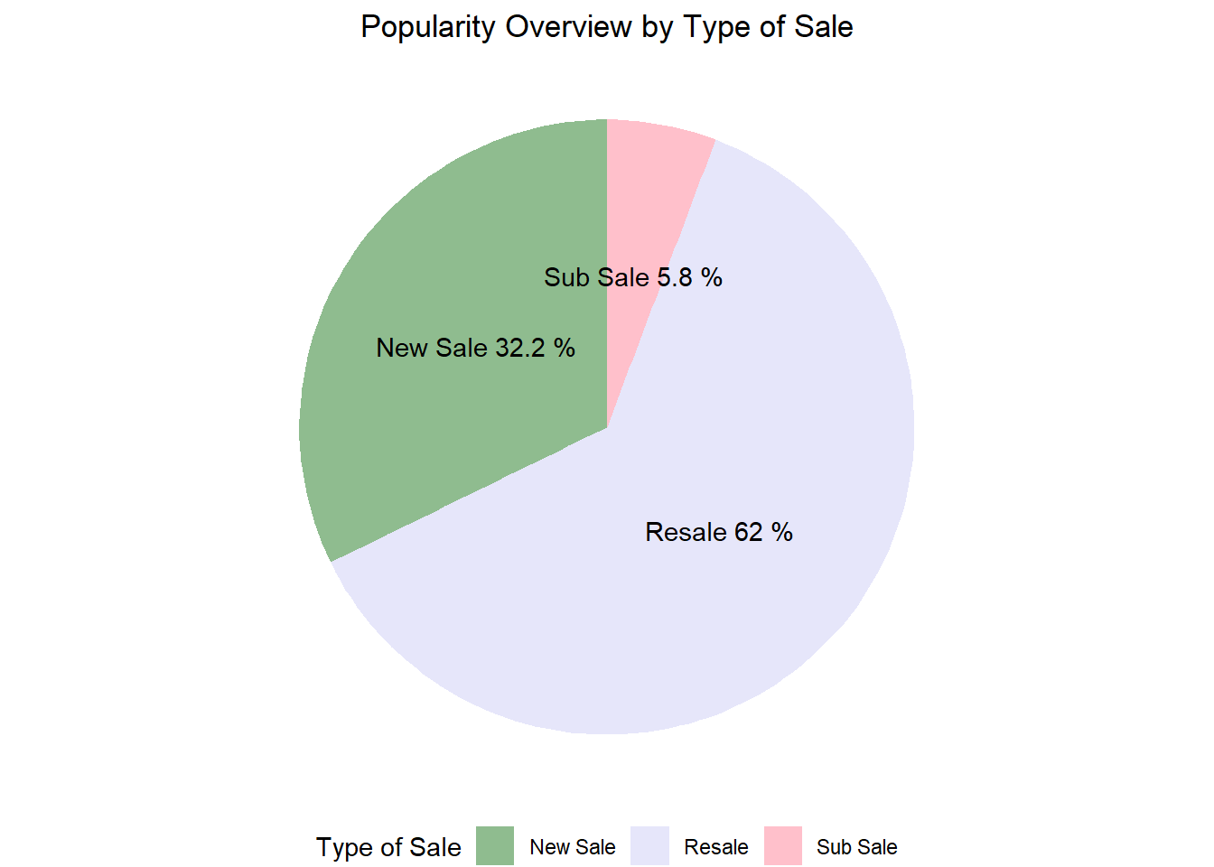
Code
# Filter for 'New Sale' transactions
new_sale_transactions <- cleaned_data %>%
  filter(`Type of Sale` == "New Sale") %>%
  count(`Property Type`, `Planning Region`) %>%
  complete(`Property Type`, `Planning Region`, fill = list(n = 0))

# heatmap for 'New Sale'
heatmap_new_sale <- ggplot(new_sale_transactions, aes(x = `Planning Region`, y = `Property Type`, fill = n)) +
  geom_tile(color = "white") +
  geom_text(aes(label = n), color = "black", size = 3, vjust = 1) +
  scale_fill_gradient(low = "white", high = "darkseagreen", name = "Transactions") +
  labs(
    title = "Popularity of New Sale Flats by Planning Region",
    x = "Planning Region",
    y = "Type of Property"
  ) +
  theme_minimal() +
  theme(
    axis.text.x = element_text(angle = 45, hjust = 1),  # Rotate x-axis labels for better readability
    legend.position = "right"  # legend position
  )

heatmap_new_sale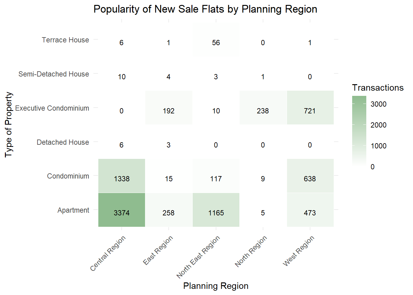
Code
# Filter for 'Resale' transactions
new_sale_transactions <- cleaned_data %>%
  filter(`Type of Sale` == "Resale") %>%
  count(`Property Type`, `Planning Region`) %>%
  complete(`Property Type`, `Planning Region`, fill = list(n = 0))

# Create the heatmap for 'Resale'
heatmap_Resale <- ggplot(new_sale_transactions, aes(x = `Planning Region`, y = `Property Type`, fill = n)) +
  geom_tile(color = "white") +
  geom_text(aes(label = n), color = "black", size = 3, vjust = 1) +
  scale_fill_gradient(low = "white", high = "lavender", name = "Transactions") +
  labs(
    title = "Popularity of Resale Flats by Planning Region",
    x = "Planning Region",
    y = "Type of Property"
  ) +
  theme_minimal() +
  theme(
    axis.text.x = element_text(angle = 45, hjust = 1),
    legend.position = "right"
  )

heatmap_Resale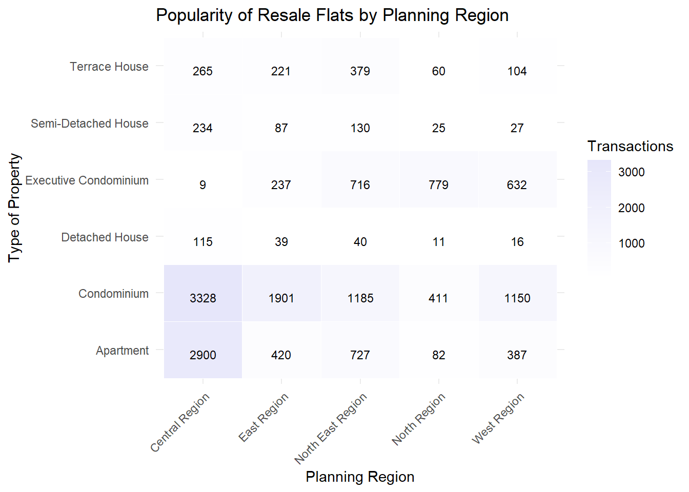
Code
# Filter for 'Sub Sale' transactions
new_sale_transactions <- cleaned_data %>%
  filter(`Type of Sale` == "Sub Sale") %>%
  count(`Property Type`, `Planning Region`) %>%
  complete(`Property Type`, `Planning Region`, fill = list(n = 0))

# Create the heatmap for 'Sub Sale'
heatmap_Sub_Sale <- ggplot(new_sale_transactions, aes(x = `Planning Region`, y = `Property Type`, fill = n)) +
  geom_tile(color = "white") +
  geom_text(aes(label = n), color = "black", size = 3, vjust = 1) +
  scale_fill_gradient(low = "white", high = "pink", name = "Transactions") +
  labs(
    title = "Popularity of Sub-sale Flats by Planning Region",
    x = "Planning Region",
    y = "Type of Property"
  ) +
  theme_minimal() +
  theme(
    axis.text.x = element_text(angle = 45, hjust = 1),
    legend.position = "right"
  )

heatmap_Sub_Sale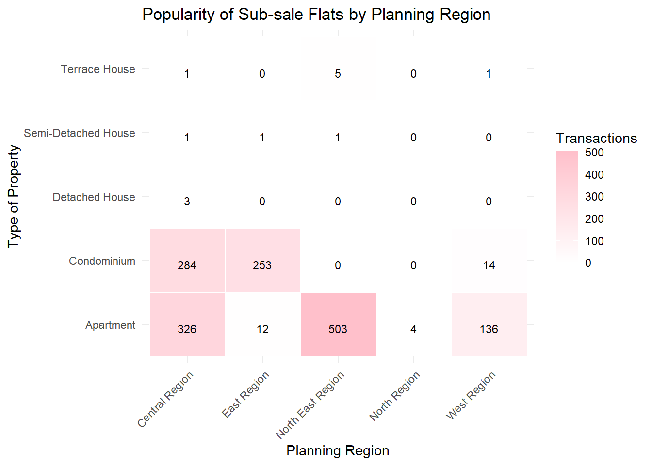
Moving forward, we will explore transaction volumes to gauge popularity. Resale properties dominate the market, accounting for 62% of transactions, followed by new sales at 32.2% and sub-sales at 5.8%. Under both resale and new sale categories, condominiums and apartments in the Central Region are the most favored, while the North Region remains the least preferred. Interestingly, resale transactions show a preference for condominiums, whereas buyers of new sales are inclined towards apartments. In the case of sub-sales, the North East Region emerges as the most popular, with the Central Region trailing behind, yet the North Region consistently ranks as the least favored across all sales types.