Code
pacman::p_load(tidytext, readtext, quanteda, tidyverse, jsonlite, igraph, tidygraph, ggraph, visNetwork, clock, graphlayouts,ggplot2)In this VAST Challenge project, we analyze the impact of SouthSeafood Express Corp’s illegal fishing on the business network. The first question explores how the network and competing businesses change due to the incident. The second question identifies which companies benefited from SouthSeafood Express Corp’s legal troubles.
pacman::p_load(tidytext, readtext, quanteda, tidyverse, jsonlite, igraph, tidygraph, ggraph, visNetwork, clock, graphlayouts,ggplot2)Direct import of the mc3.json file shows an error message indicating that there’s an invalid character in the JSON text, specifically “NaN”. As “NaN” is not recognised as a valid value, preprocessing of the JSON file to replace “NaN” is required.
# Read the JSON file as text
json_text <- readLines("data/mc3.json" ,warn = FALSE)

# Replace "NaN" with "null"
json_text_fixed <- gsub("NaN", "null", json_text)

# Write the fixed JSON text back to a file
writeLines(json_text_fixed, "data/mc3_fixed.json")
Importing preprocessed mc3_fixed.json file
mc3_data <- fromJSON("data/mc3_fixed.json")Identify the percentage of missing values within the dataset
# Function to calculate missing value percentages
calculate_missing_percentage <- function(df) {
  total_values <- nrow(df) * ncol(df)
  missing_values <- sum(is.na(df))
  missing_percentage <- (missing_values / total_values) * 100
  return(missing_percentage)
}
Missing percentage of nodes
nodes_missing_percentage <- calculate_missing_percentage(mc3_data[["nodes"]])
nodes_missing_percentage
[1] 35.11952nodes_missing_by_column <- sapply(mc3_data[["nodes"]], function(x) sum(is.na(x)) / length(x) * 100)Missing percentage of edges
links_missing_percentage <- calculate_missing_percentage(mc3_data[["links"]])
links_missing_percentage
[1] 9.059973links_missing_by_column <- sapply(mc3_data[["links"]], function(x) sum(is.na(x)) / length(x) * 100)
links_missing_by_column start_date type _last_edited_by _last_edited_date
0.1187069 0.0000000 0.0000000 0.0000000
_date_added _raw_source _algorithm source
0.0000000 0.0000000 0.0000000 0.0000000
target key end_date
0.0000000 0.0000000 99.5410000 Print missing percentages
#
print(nodes_missing_percentage)
[1] 35.11952print(nodes_missing_by_column) type country ProductServices PointOfContact
0.00000 0.00000 85.34204 85.38334
HeadOfOrg founding_date revenue TradeDescription
85.35691 85.34204 85.36847 85.34204
_last_edited_by _last_edited_date _date_added _raw_source
0.00000 0.00000 0.00000 0.00000
_algorithm id dob
0.00000 0.00000 14.65796 print(links_missing_percentage)[1] 9.059973print(links_missing_by_column) start_date type _last_edited_by _last_edited_date
0.1187069 0.0000000 0.0000000 0.0000000
_date_added _raw_source _algorithm source
0.0000000 0.0000000 0.0000000 0.0000000
target key end_date
0.0000000 0.0000000 99.5410000 Nodes Data:
ProductServices, PointOfContact, HeadOfOrg, founding_date, revenue, and TradeDescription columns have a high percentage of missing values (around 85%).
The dob column has about 14.7% missing values.
Other columns (type, country, _last_edited_by, _last_edited_date, _date_added, _raw_source, _algorithm, and id) have no missing values.
Links Data:
end_date has a very high percentage of missing values (around 99.5%).Filled missing values in HeadOfOrg with “Unknown”.
Filled missing values in revenue with 0.
Filled missing values in start_date and end_date with “Unknown”.
Handle missing values
# Select crucial columns and fill missing values where appropriate
cleaned_nodes <- mc3_data[["nodes"]] %>%
  select(id, type, country, HeadOfOrg, revenue,ProductServices,PointOfContact,founding_date,TradeDescription,dob,
         `_last_edited_by`, `_last_edited_date`, `_date_added`, `_raw_source`, `_algorithm`) %>%
  mutate(HeadOfOrg = ifelse(is.na(HeadOfOrg), "Unknown", HeadOfOrg),
         revenue = ifelse(is.na(revenue), 0, revenue))

# Handle missing values in links
# Select crucial columns and fill missing values where appropriate
cleaned_links <- mc3_data[["links"]] %>%
  select(key,source, target, type, start_date, end_date, `_last_edited_by`, `_last_edited_date`, `_date_added`, `_raw_source`, `_algorithm`) %>%
  mutate(start_date = ifelse(is.na(start_date), "Unknown", start_date),
         end_date = ifelse(is.na(end_date), "Unknown", end_date))

# Ensure proper data types
cleaned_nodes <- cleaned_nodes %>%
  mutate(
    id = as.character(id),
    type = as.character(type),
    country = as.character(country),
    HeadOfOrg = as.character(HeadOfOrg),
    revenue = as.numeric(revenue),
    `_last_edited_by` = as.character(`_last_edited_by`),
    `_last_edited_date` = as.character(`_last_edited_date`),
    `_date_added` = as.character(`_date_added`),
    `_raw_source` = as.character(`_raw_source`),
    `_algorithm` = as.character(`_algorithm`)
  )

cleaned_links <- cleaned_links %>%
 mutate(
    source = as.character(source),
    target = as.character(target),
    type = as.character(type),
    start_date = as.character(start_date),
    end_date = as.character(end_date),
    `_last_edited_by` = as.character(`_last_edited_by`),
    `_last_edited_date` = as.character(`_last_edited_date`),
    `_date_added` = as.character(`_date_added`),
    `_raw_source` = as.character(`_raw_source`),
    `_algorithm` = as.character(`_algorithm`)
)# Ensure correct data types for nodes
cleaned_nodes <- cleaned_nodes %>%
mutate(
id = as.character(id),
type = as.character(type),
country = as.character(country),
HeadOfOrg = as.character(HeadOfOrg),
revenue = as.numeric(revenue),
dob = as.POSIXct(dob, format="%Y-%m-%dT%H:%M:%S"),
`_last_edited_by` = as.character(`_last_edited_by`),
`_last_edited_date` = as.POSIXct(`_last_edited_date`, format="%Y-%m-%dT%H:%M:%S"),
founding_date=as.POSIXct(founding_date, format="%Y-%m-%dT%H:%M:%S"),
`_date_added` = as.POSIXct(`_date_added`, format="%Y-%m-%dT%H:%M:%S"),
`_raw_source` = as.character(`_raw_source`),
`_algorithm` = as.character(`_algorithm`)
)
# Ensure correct data types for links
cleaned_links <- cleaned_links %>%
mutate(
source = as.character(source),
target = as.character(target),
type = as.character(type),
start_date = as.POSIXct(start_date, format="%Y-%m-%dT%H:%M:%S"),
end_date = as.POSIXct(end_date, format="%Y-%m-%dT%H:%M:%S"),
`_last_edited_by` = as.character(`_last_edited_by`),
`_last_edited_date` = as.POSIXct(`_last_edited_date`, format="%Y-%m-%dT%H:%M:%S"),
`_date_added` = as.POSIXct(`_date_added`, format="%Y-%m-%dT%H:%M:%S"),
`_raw_source` = as.character(`_raw_source`),
`_algorithm` = as.character(`_algorithm`)
)
# Print cleaned data for inspection
glimpse(cleaned_nodes)Rows: 60,520
Columns: 15
$ id <chr> "Abbott, Mcbride and Edwards", "Abbott-Gomez", "Ab…
$ type <chr> "Entity.Organization.Company", "Entity.Organizatio…
$ country <chr> "Uziland", "Mawalara", "Uzifrica", "Islavaragon", …
$ HeadOfOrg <chr> "Émilie-Susan Benoit", "Honoré Lemoine", "Jules La…
$ revenue <dbl> 5994.73, 71766.67, 0.00, 0.00, 4746.67, 46566.67, …
$ ProductServices <chr> "Unknown", "Furniture and home accessories", "Food…
$ PointOfContact <chr> "Rebecca Lewis", "Michael Lopez", "Steven Robertso…
$ founding_date <dttm> 1954-04-24, 2009-06-12, 2029-12-15, 1972-02-16, 1…
$ TradeDescription <chr> "Unknown", "Abbott-Gomez is a leading manufacturer…
$ dob <dttm> NA, NA, NA, NA, NA, NA, NA, NA, NA, NA, NA, NA, N…
$ `_last_edited_by` <chr> "Pelagia Alethea Mordoch", "Pelagia Alethea Mordoc…
$ `_last_edited_date` <dttm> 2035-01-01, 2035-01-01, 2035-01-01, 2035-01-01, 2…
$ `_date_added` <dttm> 2035-01-01, 2035-01-01, 2035-01-01, 2035-01-01, 2…
$ `_raw_source` <chr> "Existing Corporate Structure Data", "Existing Cor…
$ `_algorithm` <chr> "Automatic Import", "Automatic Import", "Automatic…glimpse(cleaned_links)Rows: 75,817
Columns: 11
$ key <int> 0, 0, 0, 0, 0, 0, 0, 0, 0, 0, 0, 0, 0, 0, 0, 0, 0,…
$ source <chr> "Avery Inc", "Berger-Hayes", "Bowers Group", "Bowm…
$ target <chr> "Allen, Nichols and Thompson", "Jensen, Morris and…
$ type <chr> "Event.Owns.Shareholdership", "Event.Owns.Sharehol…
$ start_date <dttm> 2016-10-29, 2035-06-03, 2028-11-20, 2024-09-04, 2…
$ end_date <dttm> NA, NA, NA, NA, NA, NA, NA, NA, NA, NA, NA, NA, N…
$ `_last_edited_by` <chr> "Pelagia Alethea Mordoch", "Niklaus Oberon", "Pela…
$ `_last_edited_date` <dttm> 2035-01-01, 2035-07-15, 2035-01-01, 2035-01-01, 2…
$ `_date_added` <dttm> 2035-01-01, 2035-07-15, 2035-01-01, 2035-01-01, 2…
$ `_raw_source` <chr> "Existing Corporate Structure Data", "Oceanus Corp…
$ `_algorithm` <chr> "Automatic Import", "Manual Entry", "Automatic Imp…cleaned_nodes <- cleaned_nodes %>%
rename("last_edited_by" = "_last_edited_by",
"date_added" = "_date_added",
"last_edited_date" = "_last_edited_date",
"raw_source" = "_raw_source",
"algorithm" = "_algorithm")
cleaned_links<- cleaned_links %>%
rename("last_edited_by" = "_last_edited_by",
"date_added" = "_date_added",
"last_edited_date" = "_last_edited_date",
"raw_source" = "_raw_source",
"algorithm" = "_algorithm") We are going to tidy the type column by creating two columns “entity2,entity3”.
word_list1 <- strsplit(cleaned_nodes$type, "\\.")
max_elements1 <- max(lengths(word_list1))
word_list_padded1 <- lapply(word_list1,
function(x) c(x, rep(NA, max_elements1 - length(x))))
word_df1 <- do.call(rbind, word_list_padded1)
colnames(word_df1) <- paste0("entity", 1:max_elements1)
word_df1 <- as_tibble(word_df1) %>%
  select(entity2, entity3)
class(word_df1)
[1] "tbl_df" "tbl" "data.frame"The steps below will be used to split text in type column into two columns
word_list <- strsplit(cleaned_links$type, "\\.")
max_elements <- max(lengths(word_list))
word_list_padded <- lapply(word_list,
function(x) c(x, rep(NA, max_elements - length(x))))
word_df <- do.call(rbind, word_list_padded)
colnames(word_df) <- paste0("event", 1:max_elements)
word_df <- as_tibble(word_df) %>%
  select(event2, event3)
class(word_df)
[1] "tbl_df" "tbl" "data.frame"Since the output above is a matrix, the code chunk above is used to convert word_df into a tibble data.frame.
cleaned_nodes <- cleaned_nodes %>%
cbind(word_df1)cleaned_links <- cleaned_links %>%
cbind(word_df)The code chunk above appends the extracted columns back to edges tibble data.frame.
write_rds(cleaned_nodes, "data/rds/cleaned_nodes.rds")
write_rds(cleaned_links, "data/rds/cleaned_links.rds")
above code write into R rds file format.
By analyzing the ownership structure, we tracked changes in most influential individuals (VIP) networks over time, identifying key individuals with increasing influence.
Split the nodes into people and companies, and filter ownership-related edges
# Split the nodes into people and companies
nodes_people <- cleaned_nodes %>% filter(entity2 == "Person")
nodes_company <- cleaned_nodes %>% filter(entity2 == "Organization")# Filter the links to include only ownership-related edges
links_owns <- cleaned_links %>% filter(event2 == "Owns")nodes_people <- nodes_people %>%
rowwise() %>%
mutate('no_owns' = sum(links_owns$source == id))
nodes_people$no_owns <- as.numeric(nodes_people$no_owns)# Calculate the unique counts of 'no_owns' and their corresponding counts and percentages
owns_summary <- nodes_people %>%
group_by(no_owns) %>%
summarise(count = n()) %>%
mutate(percentage = (count / sum(count)) * 100)
# Display the summary
print(owns_summary)# A tibble: 19 × 3
no_owns count percentage
<dbl> <int> <dbl>
1 0 147 0.285
2 1 46370 89.8
3 2 4032 7.81
4 3 665 1.29
5 4 245 0.474
6 5 80 0.155
7 6 34 0.0658
8 7 21 0.0407
9 8 11 0.0213
10 9 7 0.0136
11 10 2 0.00387
12 11 4 0.00774
13 12 3 0.00581
14 13 2 0.00387
15 15 1 0.00194
16 18 2 0.00387
17 29 1 0.00194
18 91 18 0.0349
19 92 4 0.00774To define and identify influential people based on an ownership threshold. It filters the nodes to keep only those with a significant number of ownerships
# Define the threshold for 'influential'
vip_threshold <- 91

# Filter to keep only influential people and select relevant columns
vip <- nodes_people %>%
  filter(no_owns >= vip_threshold) %>%
  select(id, country, dob, last_edited_date, date_added, no_owns)

# Display the updated vip data frame
glimpse(vip)
Rows: 22
Columns: 6
Rowwise:
$ id <chr> "Kelsey Ortega", "Joseph Gentry", "Cynthia Anderson",…
$ country <chr> "n.a.", "n.a.", "n.a.", "n.a.", "n.a.", "n.a.", "n.a.…
$ dob <dttm> 1974-11-26, 1980-11-08, 1991-07-23, 2013-10-03, 1981…
$ last_edited_date <dttm> 2035-01-01, 2035-01-01, 2035-01-01, 2035-01-01, 2035…
$ date_added <dttm> 2035-01-01, 2035-01-01, 2035-01-01, 2035-01-01, 2035…
$ no_owns <dbl> 91, 91, 91, 92, 91, 92, 91, 91, 91, 91, 91, 91, 91, 9…filter the ownership connections to include only those involving these influential individuals
# Filter links_owns to keep only those connections where the source is in the vip list
vip_connections <- links_owns %>%
  filter(source %in% vip$id)%>%
  select(source, target,start_date,end_date,last_edited_date, date_added)

# Display the updated vip_connections data frame
glimpse(vip_connections)
Rows: 2,006
Columns: 6
$ source <chr> "Kelsey Ortega", "Kelsey Ortega", "Kelsey Ortega", "K…
$ target <chr> "Mitchell-Glover", "Anderson, Smith and Weber", "Orr …
$ start_date <dttm> 2017-08-11, 2028-12-13, 2016-09-18, 2034-12-16, 2032…
$ end_date <dttm> NA, NA, NA, NA, 2035-07-13, NA, NA, NA, NA, NA, NA, …
$ last_edited_date <dttm> 2035-01-01, 2035-01-01, 2035-01-01, 2035-01-01, 2035…
$ date_added <dttm> 2035-01-01, 2035-01-01, 2035-01-01, 2035-01-01, 2035…Finally, plot the network, highlighting the structure and connections of influential individuals.
# Create graph from VIP connections
g_vip <- graph_from_data_frame(d = vip_connections, directed = TRUE)

# Identify VIPs and Companies
V(g_vip)$type <- ifelse(V(g_vip)$name %in% nodes_people$id, "VIP", "Company")

# Define colors and sizes
V(g_vip)$color <- ifelse(V(g_vip)$type == "VIP", "blue", "orange")
V(g_vip)$size <- ifelse(V(g_vip)$type == "VIP", 8, 5)

# Plot the network
plot(g_vip, vertex.label = NA, vertex.size = V(g_vip)$size, edge.arrow.size = 0.5,
     vertex.color = V(g_vip)$color, main = "VIP Connections Network")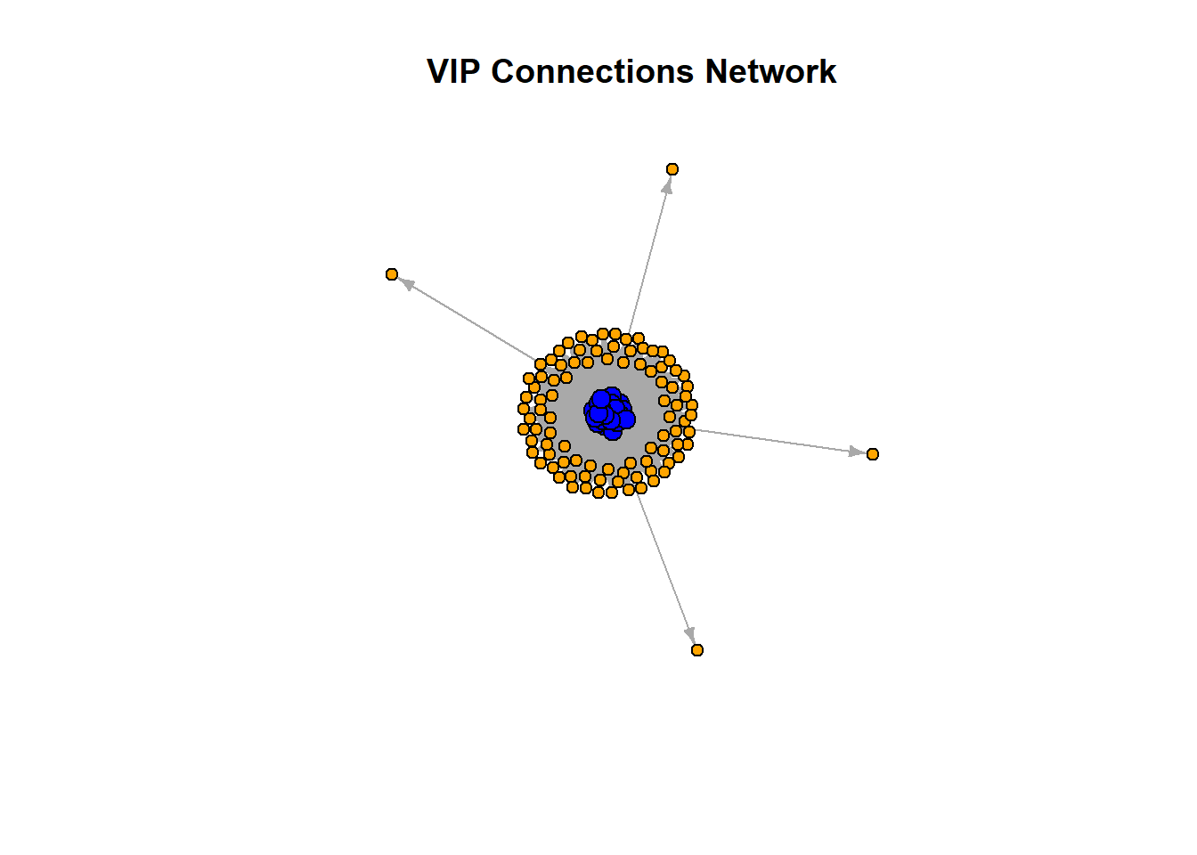
The plot represents the VIP Connections Network, with blue nodes indicating influential VIPs and orange nodes representing companies they own. Directed edges illustrate ownership, pointing from VIPs to companies. This visualization highlights the dense centrality of VIPs, showcasing their extensive control across multiple companies. By examining these connections, we can infer the structure and extent of VIP influence within the network and help FishEye identify influential individuals within the business network, highlighting ownership structures and central figures. By tracking ownership changes over time, FishEye can pinpoint who controls companies involved in illegal fishing activities.
While this plot provides a static snapshot, in the following we shall create similar plots for different time periods can reveal changes in ownership and influence over time.
Aggregate Ownership Changes by Year
change_over_time1 <- links_owns %>%
  group_by(start_date) %>%
  summarize(count = n()) %>%
  drop_na()

links_owns<- links_owns %>%
  mutate(start_year = format(start_date, "%Y"))

# Aggregate ownership changes by year
change_over_time <- links_owns %>%
  group_by(start_year) %>%
  summarize(count = n()) %>%
  drop_na()
Create plots to visualize the changes in ownership over time.
# Plot changes over time
ggplot(change_over_time, aes(x = as.numeric(start_year), y = count)) +
  geom_line() +
  geom_point() +
  labs(title = "Changes in Ownership Over Time",
       x = "Year",
       y = "Number of Ownership Changes") +
  theme_minimal()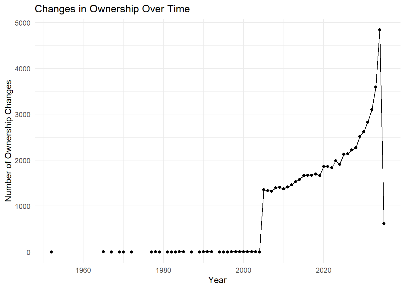
Given the significant increase in data from 2004 onwards, focusing on every 10 years from 2005 to 2035 would provide a more detailed analysis of changes in ownership and influence.
# Specify the year
filter_year <- 2005

# Filter vip_connections by start_year
vip_connections_filtered <- vip_connections %>%
  filter(format(start_date, "%Y") == filter_year)

# Create the graph object from the filtered vip_connections
g_vip_filtered <- graph_from_data_frame(d = vip_connections_filtered, directed = TRUE)

# Identify VIPs (nodes_people) and Companies
V(g_vip_filtered)$type <- ifelse(V(g_vip_filtered)$name %in% nodes_people$id, "VIP", "Company")

# Define colors and sizes
V(g_vip_filtered)$color <- ifelse(V(g_vip_filtered)$type == "VIP", "blue", "orange")
V(g_vip_filtered)$size <- ifelse(V(g_vip_filtered)$type == "VIP", 8, 5)

# Plot the network
p2005<-plot(g_vip_filtered, vertex.label = NA, vertex.size = V(g_vip_filtered)$size, edge.arrow.size = 0.5,
     vertex.color = V(g_vip_filtered)$color, main = paste("VIP Connections Network for", filter_year))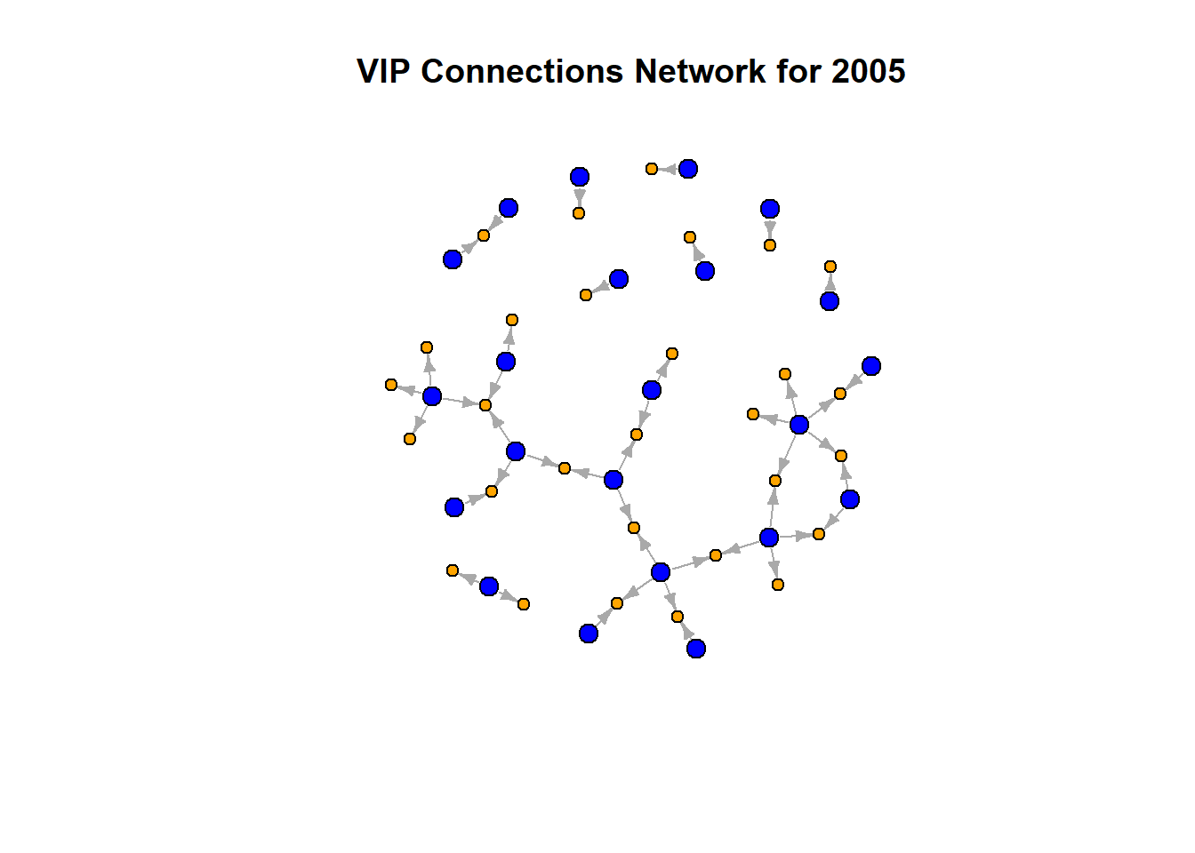
In 2005, the network shows a relatively sparse structure with a moderate number of connections. VIPs (blue nodes) are moderately interconnected, indicating a balanced distribution of influence among several key players.
# Specify the year
filter_year <- 2015

# Filter vip_connections by start_year
vip_connections_filtered_2015 <- vip_connections %>%
  filter(format(start_date, "%Y") == filter_year)

# Create the graph object from the filtered vip_connections
g_vip_filtered_2015 <- graph_from_data_frame(d = vip_connections_filtered_2015, directed = TRUE)

# Identify VIPs (nodes_people) and Companies
V(g_vip_filtered_2015)$type <- ifelse(V(g_vip_filtered_2015)$name %in% nodes_people$id, "VIP", "Company")

# Define colors and sizes
V(g_vip_filtered_2015)$color <- ifelse(V(g_vip_filtered_2015)$type == "VIP", "blue", "orange")
V(g_vip_filtered_2015)$size <- ifelse(V(g_vip_filtered_2015)$type == "VIP", 8, 5)

# Plot the network
p2015 <- plot(g_vip_filtered_2015, vertex.label = NA, vertex.size = V(g_vip_filtered_2015)$size, edge.arrow.size = 0.5,
     vertex.color = V(g_vip_filtered_2015)$color, main = paste("VIP Connections Network for", filter_year))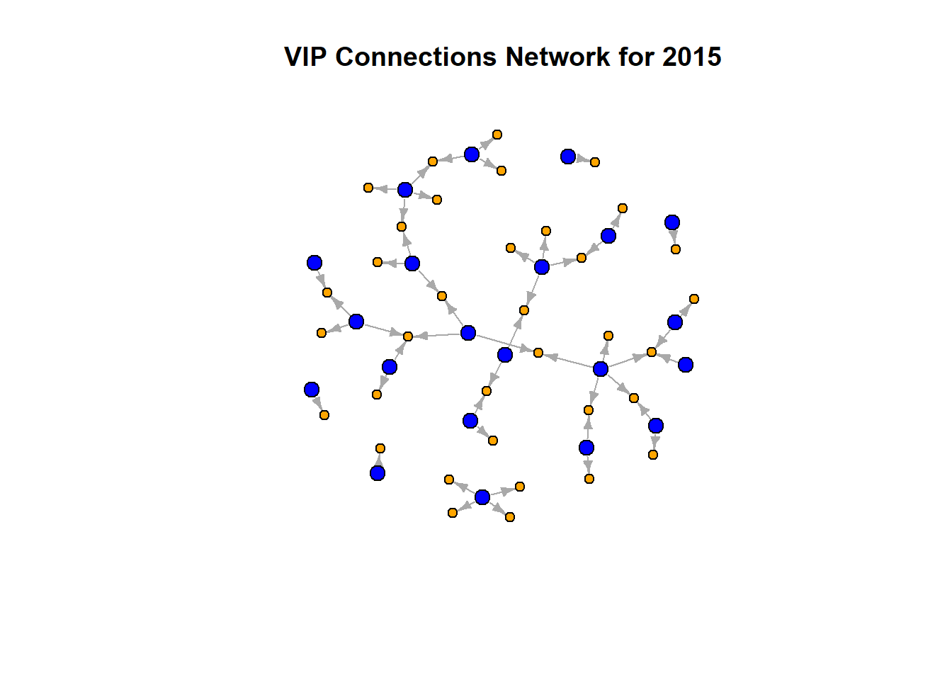
By 2015, the network has grown denser, suggesting increased interconnectedness and influence consolidation. More VIPs are connected to multiple companies (orange nodes), indicating a significant rise in their influence and control over the network.
# Specify the year
filter_year <- 2025

# Filter vip_connections by start_year
vip_connections_filtered_2025 <- vip_connections %>%
  filter(format(start_date, "%Y") == filter_year)

# Create the graph object from the filtered vip_connections
g_vip_filtered_2025 <- graph_from_data_frame(d = vip_connections_filtered_2025, directed = TRUE)

# Identify VIPs (nodes_people) and Companies
V(g_vip_filtered_2025)$type <- ifelse(V(g_vip_filtered_2025)$name %in% nodes_people$id, "VIP", "Company")

# Define colors and sizes
V(g_vip_filtered_2025)$color <- ifelse(V(g_vip_filtered_2025)$type == "VIP", "blue", "orange")
V(g_vip_filtered_2025)$size <- ifelse(V(g_vip_filtered_2025)$type == "VIP", 8, 5)

# Plot the network
p2025 <- plot(g_vip_filtered_2025, vertex.label = NA, vertex.size = V(g_vip_filtered_2025)$size, edge.arrow.size = 0.5,
     vertex.color = V(g_vip_filtered_2025)$color, main = paste("VIP Connections Network for", filter_year))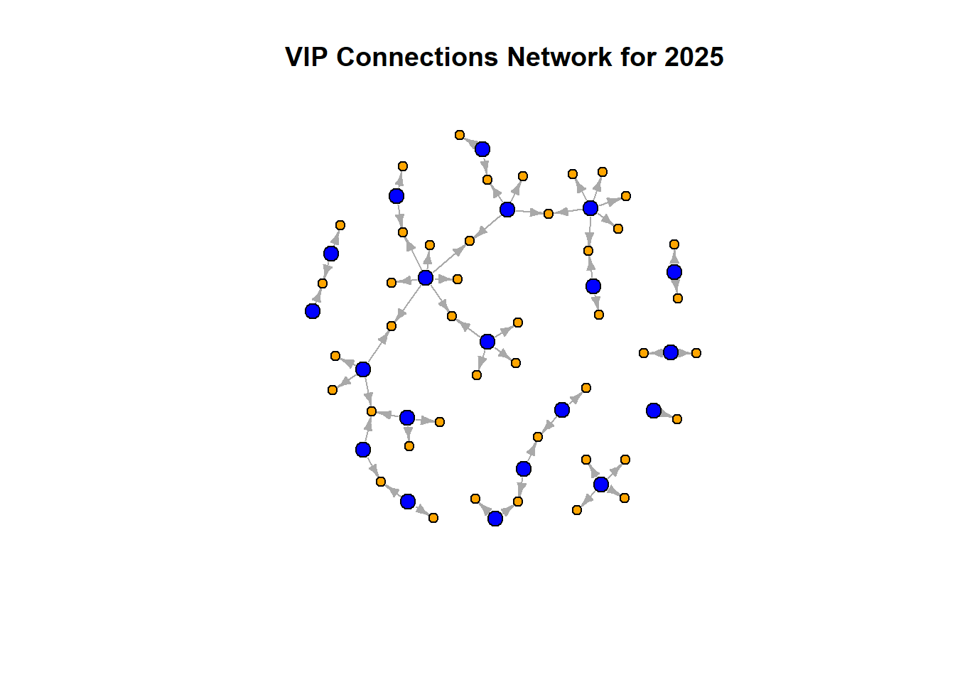
The network continues to expand in 2025, displaying even more complexity and interconnections. This period likely represents a peak in influence for several VIPs, with many of them owning shares in numerous companies, suggesting increased market control.
# Specify the year
filter_year <- 2035

# Filter vip_connections by start_year
vip_connections_filtered_2035 <- vip_connections %>%
  filter(format(start_date, "%Y") == filter_year)

# Create the graph object from the filtered vip_connections
g_vip_filtered_2035 <- graph_from_data_frame(d = vip_connections_filtered_2035, directed = TRUE)

# Identify VIPs (nodes_people) and Companies
V(g_vip_filtered_2035)$type <- ifelse(V(g_vip_filtered_2035)$name %in% nodes_people$id, "VIP", "Company")

# Define colors and sizes
V(g_vip_filtered_2035)$color <- ifelse(V(g_vip_filtered_2035)$type == "VIP", "blue", "orange")
V(g_vip_filtered_2035)$size <- ifelse(V(g_vip_filtered_2035)$type == "VIP", 8, 5)

# Plot the network
p2035 <- plot(g_vip_filtered_2035, vertex.label = NA, vertex.size = V(g_vip_filtered_2035)$size, edge.arrow.size = 0.5,
     vertex.color = V(g_vip_filtered_2035)$color, main = paste("VIP Connections Network for", filter_year))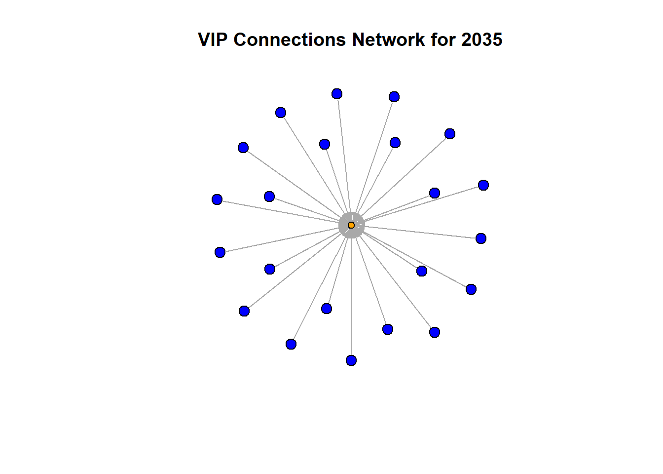
In 2035, the network structure shifts to a star-like formation, where a central VIP appears to have gained substantial influence, with direct connections to numerous companies. This indicates a significant consolidation of power and influence, where a few key players dominate the network.
Initially, influence is distributed among several key players, but over the years, it becomes concentrated among fewer individuals, leading to a highly centralized network by 2035. This centralization of power can be both an opportunity for streamlined decision-making and a risk for monopolistic control. Monitoring these changes is crucial for regulatory bodies like FishEye to ensure fair practices and prevent illegal activities within the network.
For part 1, the focus was on identifying the network associated with SouthSeafood Express Corp and visualizing how this network and competing businesses changed as a result of their illegal fishing behavior.
Locate the node representing SouthSeafood Express Corp in the network.
Create a visualization of the network associated with SouthSeafood Express Corp before any changes.
# Extract edges connected to SouthSeafood Express Corp
southseafood_edges <- cleaned_links %>%
  filter(source == "SouthSeafood Express Corp" | target == "SouthSeafood Express Corp")%>%
  select(source,target,start_date,end_date,event2)

# Ensure all nodes in the edge list are present in the vertex data frame
southseafood_nodes <- cleaned_nodes %>%
  filter(id %in% (c(southseafood_edges$source, southseafood_edges$target)))

# Join edges with nodes to ensure all nodes are present
southseafood_edges <- southseafood_edges %>%
  filter(source %in% southseafood_nodes$id & target %in% southseafood_nodes$id)

# Create graph object for the sub-network
g_southseafood <- graph_from_data_frame(d = southseafood_edges, vertices = southseafood_nodes, directed = TRUE)

# Visualize the initial network
plot(g_southseafood, vertex.label = NA, vertex.size = 5, edge.arrow.size = 0.5,
     vertex.color = "orange", main = "Network Associated with SouthSeafood Express Corp")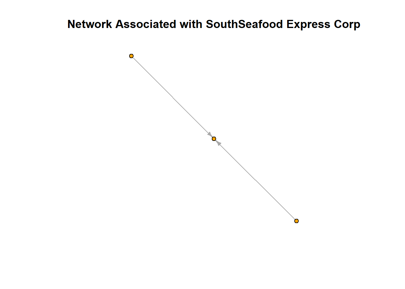
Identify and highlight competing businesses within the extracted sub-network.
competing_businesses <- cleaned_nodes %>%
filter(entity3 == "FishingCompany" & id != "SouthSeafood Express Corp")competing_edges <- cleaned_links %>%
filter(source %in% competing_businesses$id | target %in% competing_businesses$id) %>%
select(source, target, start_date, end_date, event2)
# Combine SouthSeafood Express Corp edges with competing businesses edges
combined_edges <- bind_rows(southseafood_edges, competing_edges)
# Extract the combined set of nodes
combined_nodes <- cleaned_nodes %>%
filter(id %in% c(combined_edges$source, combined_edges$target))# Create graph object for the combined network
g_combined <- graph_from_data_frame(d = combined_edges, vertices = combined_nodes, directed = TRUE)Filter the data to show the network before and after the illegal fishing incident(assume the incident happened in 2023)
Create visualizations to compare the network structure and connections before and after the incident.
# Assume the accident happened in 2023
incident_year <- 2023

# Filter edges before the incident
edges_before <- combined_edges %>%
  filter(format(start_date, "%Y") < incident_year)

# Filter edges after the incident
edges_after <- combined_edges %>%
  filter(format(start_date, "%Y") >= incident_year)

# Create graph objects for before and after the incident
g_before <- graph_from_data_frame(d = edges_before, vertices = combined_nodes, directed = TRUE)
g_after <- graph_from_data_frame(d = edges_after, vertices = combined_nodes, directed = TRUE)Identify and highlight significant changes in connections and structure due to the illegal fishing behavior and subsequent closure.
par(mfrow = c(2, 1))

plot_before <- ggraph(g_before, layout = "fr") +
  geom_edge_link(aes(edge_alpha = 0.8), show.legend = FALSE, color = "gray", width = 1) +
  geom_node_point(aes(color = ifelse(name == "SouthSeafood Express Corp", "SouthSeafood",
                                     ifelse(type == "Entity.Organization.FishingCompany", "FishingCompany", "Other"))),
                  size = 3, alpha = 0.6, show.legend = TRUE) + # Adjusted alpha for transparency
  scale_color_manual(values = c("SouthSeafood" = "red", "FishingCompany" = "blue", "Other" = "orange"),
                     name = "Type") + # Shortened legend title
  theme_void() +
  theme(legend.position = "bottom") +
  labs(title = "Network Before Incident")

# Show the plot for the network before the incident
plot_before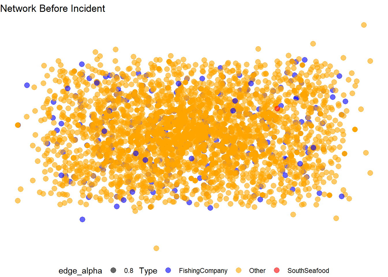
plot_after <- ggraph(g_after, layout = "fr") +
  geom_edge_link(aes(edge_alpha = 0.8), show.legend = FALSE, color = "gray", width = 1) +
  geom_node_point(aes(color = ifelse(name == "SouthSeafood Express Corp", "SouthSeafood",
                                     ifelse(type == "Entity.Organization.FishingCompany", "FishingCompany", "Other"))),
                  size = 3, alpha = 0.6, show.legend = TRUE) + # Adjusted alpha for transparency
  scale_color_manual(values = c("SouthSeafood" = "red", "FishingCompany" = "blue", "Other" = "orange"),
                     name = "Type") + # Shortened legend title
  theme_void() +
  theme(legend.position = "bottom") +
  labs(title = "Network After Incident")

# Show the plot for the network after the incident
plot_after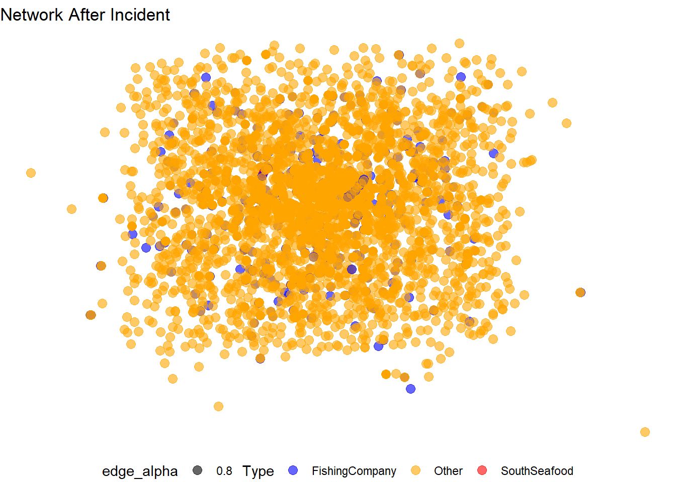
Observations:
The number of blue nodes (fishing companies) appears to have decreased.
SouthSeafood Express Corp (red node) remains central but its connections might have changed, indicating possible impact from the incident.
For part 2, since we cannot use revenue data over time, we will focus on identifying which companies potentially benefited from SouthSeafood Express Corp’s legal troubles by analyzing changes in network centrality measures.
# Calculate degree centrality before the incident
degree_before <- degree(g_before, mode = "all")

# Calculate degree centrality after the incident
degree_after <- degree(g_after, mode = "all")

# Combine degree centrality measures into a data frame
centrality_change <- data.frame(
  id = names(degree_before),
  degree_before = degree_before,
  degree_after = degree_after
)

# Calculate the change in degree centrality
centrality_change <- centrality_change %>%
  mutate(change = degree_after - degree_before)

# Display companies with the most positive change in degree centrality
top_beneficiaries <- centrality_change %>%
  arrange(desc(change)) %>%
  head(10)

print(top_beneficiaries)
id degree_before degree_after change
Anderson-Roberts Anderson-Roberts 0 36 36
Hall, Hartman and Hall Hall, Hartman and Hall 0 30 30
Kirk Inc Kirk Inc 0 18 18
Watson-Gray Watson-Gray 0 18 18
Parker Inc Parker Inc 0 17 17
Mullins-Carrillo Mullins-Carrillo 0 15 15
Torres, Ross and Brown Torres, Ross and Brown 0 14 14
Byrd and Sons Byrd and Sons 0 13 13
Haynes-Lucero Haynes-Lucero 0 13 13
Lutz-Fleming Lutz-Fleming 0 13 13# Merge with cleaned_nodes to get the entity type
top_beneficiaries_info <- top_beneficiaries %>%
left_join(cleaned_nodes, by = c("id" = "id")) %>%
select(id, change,entity3)
# Display the entity type of top beneficiaries
print(top_beneficiaries_info) id change entity3
1 Anderson-Roberts 36 FishingCompany
2 Hall, Hartman and Hall 30 FishingCompany
3 Kirk Inc 18 FishingCompany
4 Watson-Gray 18 FishingCompany
5 Parker Inc 17 FishingCompany
6 Mullins-Carrillo 15 FishingCompany
7 Torres, Ross and Brown 14 FishingCompany
8 Byrd and Sons 13 FishingCompany
9 Haynes-Lucero 13 FishingCompany
10 Lutz-Fleming 13 FishingCompany# Bar plot of top beneficiaries
ggplot(top_beneficiaries_info, aes(x = reorder(id, change), y = change)) +
geom_bar(stat = "identity", fill = "lightblue") +
coord_flip() +
theme_minimal() +
labs(title = "Top Beneficiaries by Change in Degree Centrality",
x = "Company",
y = "Change in Degree Centrality",
fill = "Entity Type") +
theme(legend.position = "none")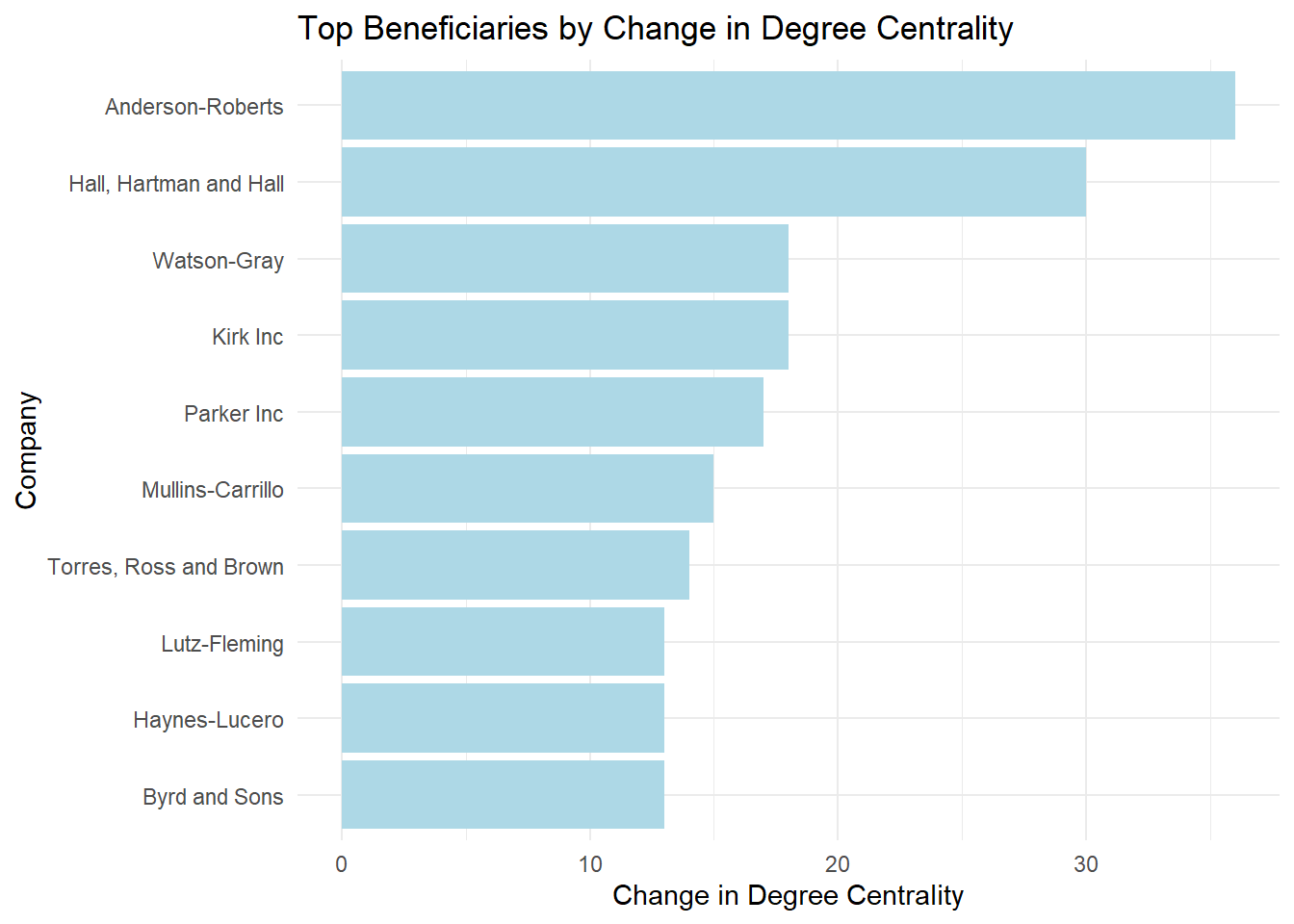
The results show that the top beneficiaries, all classified as fishing companies, significantly increased their network centrality following SouthSeafood Express Corp’s legal troubles. Anderson-Roberts, Hall, Hartman and Hall, and Kirk Inc., among others, saw the largest gains, suggesting they capitalized on the shift in the network’s structure.